Multiple Regression Analysis

Multiple regression is a statistical technique that can be used to analyze the relationship between a single dependent variable and several independent variables. The objective of multiple regression analysis is to use the independent variables whose values are known to predict the value of the single dependent value. Unlike single linear regression, in multiple linear correlation and regression, we use additional independent variables that help us better explain or predict the dependent variable (Y).

Multiple Regression Analysis

The general descriptive form of a multiple linear equation is shown in formula below. We use k to represent the number of independent variables. So k can be any positive integer. Each predictor value is weighed, the weights denoting their relative contribution to the overall prediction.

where:
a is the intercept, the value of Y when all the X’s are zero is the amount by which Y changes when that particular increases by one unit, with the values of all other independent variables held constant.

Normally linear regression analysis describes and testes the relationship between a dependent variable, and a single independent variable, X. The relationship between and X is graphically portrayed by a line. When there are two independent variables, the regression equation is

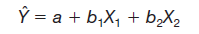
This approach can be applied to analyze multivariate time series data when one of the variables is dependent on a set of other variables. We can model the dependent variable Y on the set of independent variables. At any time instant when we are given the values of the independent variables, we can predict the value of Y from the first equation.

In time series analysis, it is possible to do regression analysis against a set of past values of the variables. This is known as autoregression (AR). Let us consider n variables. We have a time series corresponding to each variable.

If a multiple regression analysis includes more than two independent variables, we cannot use a graph to illustrate the analysis since graphs are limited to three dimensions. To illustrate the interpretation of the intercept and the two regression coefficients, suppose a vehicle’s mileage per gallon of gasoline is directly related to the octane rating of the gasoline being used (X1) and inversely related to the weight of the automobile (X2). Assume that the regression equation is:

The intercept value of 6.3 indicates the regression equation intersects the Y-axis at 6.3 when both X1 and X2 and are zero. Of course, this does not make any physical sense to own an automobile that has no (zero) weight and to use gasoline with no octane. It is important to keep in mind that a regression equation is not generally used outside the range of the sample values.

The b1 of 0.2 indicates that for each increase of 1 in the octane rating of the gasoline, the automobile would travel 2/10 of a mile more per gallon, regardless of the weight of the vehicle. The value of b2 value of -0.001 reveals that for each increase of one pound in the vehicle’s weight, the number of miles travelled per gallon decreases by 0.001, regardless of the octane of the gasoline being used. As an example, an automobile with 92-octane gasoline in the tank and weighing 2,000 pounds would travel an average 22.7 miles per gallon, found by: